Table Of Contents

Description of the model
- (MM, A)limepy: (Multi-Mass, Anisotropic) Lowered Isothermal Model Explorer in Python

Previous topic

Next topic

This Page

Description of the model¶

(MM, A)limepy: (Multi-Mass, Anisotropic) Lowered Isothermal Model Explorer in Python¶

Isotropic models¶

The isotropic distribution functions are defined as (Gomez-Leyton & Velazquez 2014)

$f_g(E) = \displaystyle \begin{cases} A\exp(E), &g=0 \\ \displaystyle A\exp(E)P(g, E), &g>1 \end{cases}$

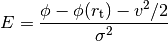where $\displaystyle E = \frac{\phi - \phi(r_{\rm t}) - v^2/2}{\sigma^2}$ , $\sigma$ is a velocity scale, $0 < \phi-\phi(r_{\rm t}) <W_0/\sigma^2$ is the (positive) potential and $P(s,x)$ is the regularised lower incomplete gamma function $P(s,x) = \gamma(s,x)/\Gamma(x)$ . For some integer values of g several well known models are found

g = 0 : Woolley (1954)
g = 1 : King (1966)
g = 2 : Wilson (1975)

Anisotropic models¶

Radial anisotropy a la Michie (1963) can be included as follows

$f_g(E, J^2) = \exp(-J^2)f_g(E),$

where $J^2 = (rv_t)^2/(2r_{\rm a}^2\sigma^2)$ , here $r_{\rm a}$ is the user-defined anisotropy radius.

Multi-mass model¶

Multi-mass models are found by summing the DFs of individual mass components and adopting for each component (following Gunn & Griffin (1979))

$\sigma_j &\propto \mu_j^{-\delta}\\ r_{{\rm a},j} &\propto \mu_j^{\eta}$

where $\mu_j = m_j/\bar{m}$ and $\bar{m}$ is the central density weighted mean mass.